Guides
Stock selection rules
On this page8
A stock-selection rule is a table of True and False: one row per day, one column per stock, True meaning hold it that day. The tables data.get() returns are FinlabDataFrames: everything you know from Pandas works, plus functions made for picking stocks, and data of different frequencies lines up on its own.
New to Pandas? Start with Pandas for strategies.
Compare a whole table in one line
A comparison works on every cell of the table at once:
from finlab import data

data.set_market('us')
close = data.get('price:adj_close')

# Closing price between $10 and $100
between_10_100 = (close > 10) & (close < 100)
close Closing price | AAPL | MSFT | NVDA | |
|---|---|---|---|
| 10/27 | 98 | 51 | 120 |
| 10/28 | 101 | 50 | 118 |
| 10/29 | 104 | 49 | 121 |
| 10/30 | 103 | 52 | 117 |
close.average(60) 60-day average | AAPL | MSFT | NVDA | |
|---|---|---|---|
| 10/27 | 100 | 52 | 115 |
| 10/28 | 100 | 51 | 116 |
| 10/29 | 101 | 51 | 117 |
| 10/30 | 101 | 51 | 118 |
position What to hold | AAPL | MSFT | NVDA | |
|---|---|---|---|
| 10/27 | False | False | True |
| 10/28 | True | False | True |
| 10/29 | True | False | True |
| 10/30 | True | True | False |
What you can use:
| Kind | Operators |
|---|---|
| Arithmetic | + - * / |
| Comparison | > >= == < <= |
| Logic | & (and), | (or), ~ (not) |
Mix daily and quarterly data directly
Prices change daily and financial statements quarterly. A FinlabDataFrame aligns them before computing, with no reindex needed:
| What | How it aligns |
|---|---|
| Dates (index) | Union of dates; a missing date takes the most recent value (forward fill) |
| Stocks (columns) | Intersection; a stock with data on only one side is dropped |
from finlab import data

data.set_market('us')
close = data.get('price:adj_close')                            # daily
net_income = data.get('us_income_statement:net_income')        # quarterly
total_assets = data.get('us_balance_sheet:total_assets')       # quarterly
roa = net_income / total_assets[total_assets > 0]

cond1 = close > 50
cond2 = roa > 0
cond_1_2 = cond1 & cond2
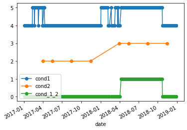
For a single stock: cond1 changes daily, cond2 only when a new quarterly report is filed, and cond_1_2 is True only when both are:
Take the top names by rank
is_largest(n) picks the n largest values on each date; is_smallest(n) the n smallest:
roe.is_largest(3) One day, six stocks- AAPL 18.2% True
- KO 6.1% False
- NVDA 24.5% True
- MSFT 11.8% False
- F 3.4% False
- JPM 15.0% True
from finlab import data

data.set_market('us')
net_income = data.get('us_income_statement:net_income')
total_assets = data.get('us_balance_sheet:total_assets')
roa = net_income / total_assets[total_assets > 0]

good_stocks = roa.is_largest(10)   # top 10 ROA on each date
The result is a boolean table with one column per stock, True for the 10 selected. Quarterly data is converted to filing dates first, so the rows are the dates reports became public and each date only compares values already disclosed.
marketcap = data.get('etl:us_market_value')
equity = data.get('us_balance_sheet:total_stockholders_equity')
pb = marketcap / equity[equity > 0]   # price-to-book, positive equity only

cheap_stocks = pb.is_smallest(10)     # 10 lowest P/B
To see each day's threshold, such as the 90th percentile, use quantile_row:
data.get('price:adj_close').quantile_row(0.9) # 90th percentile of prices each daySet entries and exits
entries.hold_until(exits) buys when the entry signal is True and holds until the exit signal is True.
buyBuy signalsellSell signalbuy.hold_until(sell)Holdingfrom finlab import data
data.set_market('us')
close = data.get('price:adj_close')
buy = close > close.average(5) # enter above the 5-day average
sell = close < close.average(20) # exit below the 20-day average
position = buy.hold_until(sell)close.average(n) is the n-period moving average; a stock gets NaN when fewer than half of the values in the window are available.
Plot a rule to check it
Pick one stock and draw the close, the average and the rule together:
import matplotlib.pyplot as plt

sma = close.average(10)
cond = close > sma

ax = close.loc['2025', 'AAPL'].plot(label='close')
sma.loc['2025', 'AAPL'].plot(ax=ax, label='sma')
cond.loc['2025', 'AAPL'].astype(int).plot(ax=ax, secondary_y=True, label='cond')
ax.legend(loc='upper left')
plt.show()
Common hold_until parameters:
| Parameter | What it does | Example |
|---|---|---|
nstocks_limit | The most stocks held at once; rotates when there are more entries | buy.hold_until(sell, nstocks_limit=5) |
rank | Which entries win when there are more than the limit (larger first) | buy.hold_until(sell, rank=-pb) |
stop_loss | Stop-loss percentage | buy.hold_until(sell, stop_loss=0.1) |
take_profit | Take-profit percentage | buy.hold_until(sell, take_profit=0.2) |
A complete strategy: enter above the 20-day average, exit below the 60-day average, hold at most 10 stocks, lowest price-to-book first.
from finlab import data
from finlab.backtest import sim

data.set_market('us')
close = data.get('price:adj_close')
marketcap = data.get('etl:us_market_value')
equity = data.get('us_balance_sheet:total_stockholders_equity')
pb = marketcap / equity[equity > 0]

entries = close > close.average(20)
exits = close < close.average(60)

position = entries.hold_until(exits, nstocks_limit=10, rank=-pb)
sim(position)
When exit signals are sparse (exit_mode)
Entry signals are always events: they count only on their own dates. When exits come from sparser data (quarterly reports, weekly or monthly conditions), exit_mode decides what dates without an exit value mean:
'state'(default): an exit is a lasting state; a date without a value takes the previous date's. A quarterly condition stays in force until the next report, and no entry happens meanwhile even if the entry signal isTrue. Theexitdates must be sorted oldest first, or aValueErroris raised; callexit.sort_index()first.'event': an exit counts only on the datesexithas; other dates mean no exit.
In both modes NaN means no exit. When exit has a row for every entry date, both modes give the same result.
To find the day each holding started or ended, use is_entry() and is_exit():
position = data.get('price:adj_close').is_largest(10)
entry_signals = position.is_entry()   # True on the day a holding starts
exit_signals = position.is_exit()     # True on the day it ends
Trends: rising, falling, several days in a row
| Write | Meaning |
|---|---|
close.rise(10) | Higher than 10 periods ago |
close.fall(10) | Lower than 10 periods ago |
cond.sustain(window, count) | True in at least count of the last window periods (every period when count is left out) |
from finlab import data

data.set_market('us')
close = data.get('price:adj_close')

close.rise(10)               # higher than 10 days ago?
close.rise().sustain(2)      # rising 2 days in a row
close.rise().sustain(3, 2)   # rising on 2 of 3 days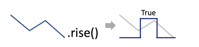
Remove the influence of size or industry
In multi-factor screens, factors are often correlated. A cheap-valuation factor (high earnings yield, low P/E) may simply be selecting small caps. Neutralization uses a cross-sectional regression to remove a factor's influence and keep the signal itself.
neutralize(factors) regresses on the factors you give and returns the residuals:
import numpy as np
from finlab import data

data.set_market('us')
close = data.get('price:adj_close')
raw_close = data.get('price:close')                  # unadjusted price for valuation
eps = data.get('us_income_statement:eps_diluted')
marketcap = data.get('etl:us_market_value')

factor = eps.rolling(4).sum() / raw_close             # trailing-12-month earnings yield
size = np.log(marketcap).replace([np.inf, -np.inf], np.nan)   # log market cap, finite values only

neutralized = factor.neutralize(size)                 # remove market-cap influence
Pass several factors as a list, or as a named dict (easier to debug):
volatility = (close / close.shift(1) - 1).rolling(60).std()   # 60-day volatility

neutralized = factor.neutralize([size, volatility])
neutralized = factor.neutralize({
    'size': size,
    'size2': size**2,
    'volatility': volatility,
})
neutralize_industry() regresses on industry and returns the residuals. Pass the classification as categories, a DataFrame with symbol and category columns. For US stocks, use the sectors in us_company_profile:
from finlab import data

profile = data.get('us_company_profile')
sectors = profile[['symbol', 'sector']].rename(columns={'sector': 'category'})

neutralized = factor.neutralize_industry(categories=sectors)   # remove sector effects
Or your own classification:
import pandas as pd

custom_cats = pd.DataFrame(
    {'symbol': ['AAPL', 'MSFT', 'JPM'], 'category': ['Hardware', 'Software', 'Banks']}
)
neutralized = factor.neutralize_industry(categories=custom_cats)
Neutralized factors work directly with rank(), is_largest() and the other selection functions, so the stocks picked reflect the factor rather than size or industry.
Other useful functions
Sector statistics
groupby_category() covers the Taiwan market only. For US sector statistics, use the sector accessor with a symbol-to-sector mapping; each stock receives its sector's statistic:
from finlab import data

data.set_market('us')
marketcap = data.get('etl:us_market_value')
equity = data.get('us_balance_sheet:total_stockholders_equity')
pb = marketcap / equity[equity > 0]

profile = data.get('us_company_profile')
sectors = dict(zip(profile['symbol'], profile['sector']))

sector_pb = pb.sector(sectors).median()
sector_pb['AAPL'].plot()   # median P/B of AAPL's sector (Technology)
Turn a report period into filing dates: index_str_to_date()
Converts a quarterly index to the dates the reports were filed; each company's value takes effect on its own filing date.
| Before | After |
|---|---|
| 2024-US-Q3 (US quarterly report) | Each company's SEC filing date, e.g. 2024-11-01 for AAPL |
from finlab import data

data.set_market('us')
data.get('us_income_statement:revenue').index_str_to_date()
data.get('us_balance_sheet:cash_and_cash_equivalents').index_str_to_date()
You rarely call it yourself: operators, is_largest(), rank(axis=1) and the other cross-sectional methods convert quarterly data automatically.
Turn a plain Pandas table into a FinlabDataFrame
What data.get() returns already is one. For a DataFrame you built:
import pandas as pd
from finlab.dataframe import FinlabDataFrame

df = pd.DataFrame()
df_finlab = FinlabDataFrame(df)
Every function and parameter is in the FinlabDataFrame API.
Next steps
- Backtesting Hand the rule to
sim(): rebalancing, stops and the trade log. - Technical indicators RSI, KD and MACD with
data.indicator(). - Download data Find the fundamentals and filings your rule needs.
- Strategy examples See complete strategies built from these rules.
Was this page helpful?